
5 Iterations (small)
an oil painting of a snowy mountain village

5 Iterations (small)
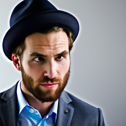
a man wearing a hat

5 Iterations (small)
a rocket ship
To start working with diffusion, we want to first set up our project so that we have some text embeddings and pretrained diffusion models that we can use to run our experiments. We use the text prompt embeddings and DeepFloyd models as specified by the project spec, and we visualize some of these here. Note that we use the default seed of $180$ for all of our experiments.

5 Iterations (small)
an oil painting of a snowy mountain village

5 Iterations (small)
a man wearing a hat

5 Iterations (small)
a rocket ship
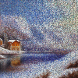
5 Iterations
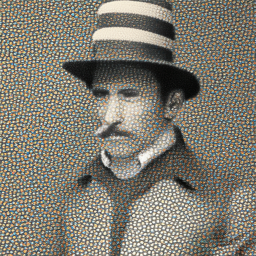
5 Iterations
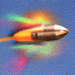
5 Iterations

20 Iterations (small)

20 Iterations (small)

20 Iterations (small)
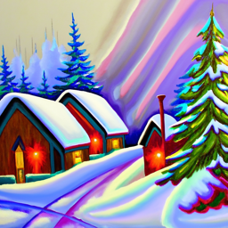
20 Iterations
20 Iterations

20 Iterations
First, we implement the forward Gaussian process in diffusion. This is defined as: \[ q(x_t|x_0) = \mathcal{N}(x_t; \sqrt{\overline{\alpha}} x_0, (1 - \overline{\alpha})I) \] \[ x_t = \sqrt{\overline{\alpha}} x_0 + \sqrt{1 - \overline{\alpha}} \epsilon, \epsilon \sim \mathcal{N}(0, 1) \]
After implementing the forward function, we show the results for $t \in [250, 500, 750]$:

Original Campanile

$t = 250$

$t = 500$

$t = 750$
Next, we implement the naive denoising process that we've learned throughout the semester: a simple Gaussian blur filter with kernel size $9$. These are expected to have poor results, but serve as our baseline:


$t = 250$


$t = 500$


$t = 750$
We can now use the pre-trained DeepFloyd diffusion model's U-Net to directly denoise the images in one step. Here, we use the time-step $t$ and the prompt "a high quality photo" as conditioning inputs.


$t = 250$
Noisy, One-Step Denoised, Original


$t = 500$
Noisy, One-Step Denoised, Original


$t = 750$
Noisy, One-Step Denoised, Original
We achieve much better results! But at higher noise, we still run into issues since we are trying to subtract a large amount of noise at once. Instead, we can use an iterative process, which is how diffusion is designed to be used. Using the original differential equations behind diffusion, we know that we can skip timesteps (strided), which will make our computation much more efficient. To go from $x_t$ to $x_t'$, we can use the following equation: \[ x_t' = \frac{\sqrt{\overline{\alpha_{t'}}}\beta_t}{1 - \overline{\alpha_{t'}}}x_0 + \frac{\sqrt{\alpha_t}(1 - \overline{\alpha_{t'}})}{1 - \overline{\alpha_t}}x_t + v_\sigma \] DeepFloyd also predicts this final variance term for us, which we can use to add noise back. We use a strided schedule skipping every 30 timesteps, and show select results below:

$t = 90$

$t = 240$

$t = 390$

$t = 540$

$t = 690$

Original Image

Iteratively Denoised

One-Step Denoising

Gaussian Denoising
We can also generate images from scratch using this iterative denoising method! We start with pure noise at i_start = 0,
and then iteratively denoise the image. We show the results below:

Sample 1

Sample 2

Sample 3

Sample 4

Sample 5
To improve the image quality, we use the Classifier-Free Guidance (CFG) method. This method computes two noise estimates, one conditional and one unconditional. Then the new noise estimate it: \[ \epsilon = \epsilon_u + \gamma (\epsilon_c - \epsilon_u) \] The unconditional prompt is just "" and the conditional prompt is "a high quality photo". We show the results below for $\gamma = 7$:

Sample 1

Sample 2

Sample 3

Sample 4

Sample 5
We can also perform interesting edits to images using diffusion. For example, we can add some noise to the image, then yank it back into the image manifold without extra conditioning. Here are some results for $i_\text{start} \in [1, 3, 5, 7, 10, 20]$:

i = 1

i = 3

i = 5

i = 7

i = 10

i = 20

Original

i = 1

i = 3

i = 5

i = 7

i = 10

i = 20

Original

i = 1

i = 3

i = 5

i = 7

i = 10

i = 20

Original
We can also perform edits on hand-drawn and web images. These are interesting because they start as being non-realistic and end up more natural in the image manifold. We show the results below:

i = 1

i = 3

i = 5

i = 7

i = 10

i = 20

Original

i = 1

i = 3

i = 5

i = 7

i = 10

i = 20

Original

i = 1

i = 3

i = 5

i = 7

i = 10

i = 20

Original
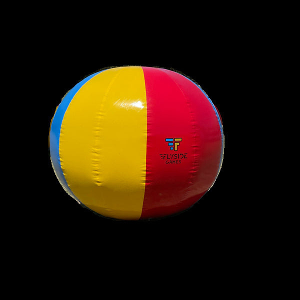
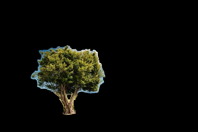
Following the RePaint paper, we can use binary masks to inpaint images. We use the following: \[ x_t \leftarrow \vec{m}x_t + (1 - \vec{m})\text{forward}(x_\text{orig}, t) \] This replaces everything in the edit mask alone, but replaces the rest of the image with the forward processed image. We show the results below:

Original

Mask

Area to Fill

Inpainted Version

Original

Mask
Area to Fill

Inpainted Version

Inpainted Version 2

Original

Mask
Area to Fill

Inpainted Version

Inpainted Version 2
We now want to guide our image generation with a text prompt. This adds control to the manifold using natural language, and specifically the text embedding space that we are sampling from. We replace the "a high quality photo" prompt with "a rocket ship" and visualize the results below:

Noise Level 1

Noise Level 3

Noise Level 5

Noise Level 7

Noise Level 10

Noise Level 20

Original

Noise Level 1

Noise Level 3

Noise Level 5

Noise Level 7

Noise Level 10

Noise Level 20

Original

Noise Level 1

Noise Level 3

Noise Level 5

Noise Level 7

Noise Level 10

Noise Level 20

Original
From here, we can do even more cool things and create visual illusions with diffusion!
One such example is visual anagrams, where originally an image might look like
an oil painting of people around a campfire, but flipped
it will look like an oil painting of an old man.
To do this, we will compute two noise estimates at each time-step, one for the original
image and one for the flipped image. We then combine these two noise estimates to create
the final noise estimate.
\[
\epsilon_1 = \text{U-Net}(x_t, t, p_1)
\]
\[
\epsilon_2 = \text{flip}(\text{U-Net}(\text{flip}(x_t), t, p_2))
\]
\[
\epsilon = (\epsilon_1 + \epsilon_2) / 2
\]
where $p_1$ and $p_2$ are the prompts for the original and flipped images, respectively.
Here are some results:

an oil painting of people around a campfire

an oil painting of an old man

an oil painting of people around a campfire

an oil painting of an old man

an oil painting of a snowy mountain village

a photo of the amalfi coast

a photo of a hipster barista

a man wearing a hat
Finally, we can implement Factorized Diffusion and create hybrid images like in Project 2. Here, we use the following: \[ \epsilon_1 = \text{U-Net}(x_t, t, p_1) \] \[ \epsilon_2 = \text{U-Net}(x_t, t, p_2) \] \[ \epsilon = f_\text{lowpass}(\epsilon_1) + f_\text{highpass}(\epsilon_2) \] We use a Gaussian blur with kernel size $9$. Here are some results:

a lithograph of a skull
a lithograph of waterfalls

an oil painting of an old man
an oil painting of a snowy mountain village

an oil painting of an old man
an oil painting of a snowy mountain village

an oil painting of an old man
an oil painting of a snowy mountain village

a man wearing a hat
a photo of the amalfi coast
We implement the simple building blocks for the U-Net, and perform a few sanity checks within the code to ensure correctness. From here, we are ready to train a one-step denoiser.
We optimize over the objective:
\[
\mathcal{L} = \mathbb{E}_{z, x} ||D_\theta (z) - x ||^2
\]
and generate $z$ from $x$ as follows:
\[
z = x + \sigma \epsilon, \epsilon \sim \mathcal{N}(0, I)
\]
We show some training samples for the NoisyMNIST dataset
below:
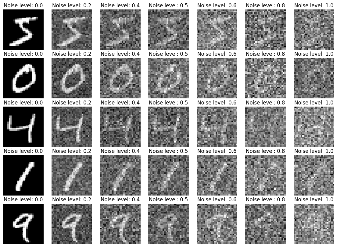
Noisy MNIST Dataset
We train a denoiser to recover an image from noise level $\sigma = 0.5$. We use hidden dimension $d = 128$ and Adam with learning rate $1e-4$. We show the training loss below:
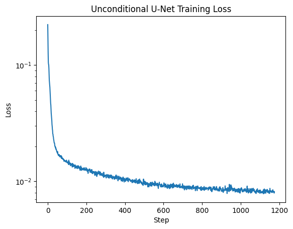
One-Step Denoiser Training Loss
We show some results below for the denoiser, once at epoch 1 and once at 5:
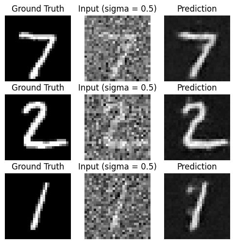
Epoch 1
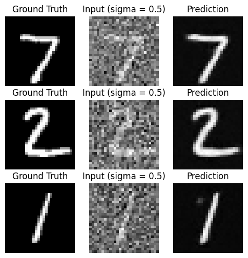
Epoch 5
We also evaluate how our denoiser does on other noise levels. Here are some results:

Out of distribution testing
From here, we want to train a full diffusion model. Instead of a separate U-Net model for every time-step, we simply train it to be conditioned on the time-step. We use $T = 300$ for the max time-steps and use a similar approach to Part A by adding fully-connected blocks for embedding the time-step.
We add an exponential learning rate scheduler, with a smaller learning rate of $1e-3$. Here is the training loss:
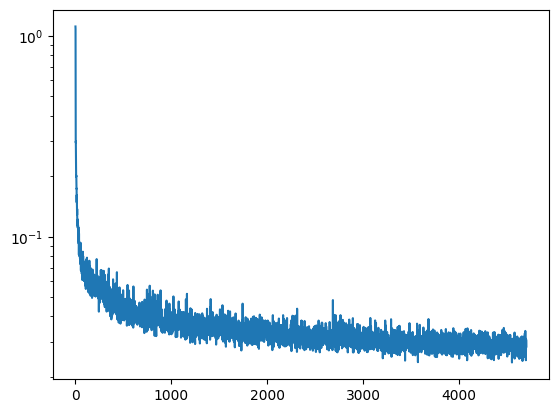
Time-Conditioned DDPM Training Loss
We also visualize some sampling results at epoch 5 and epoch 20.
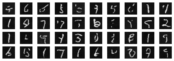
Epoch 5
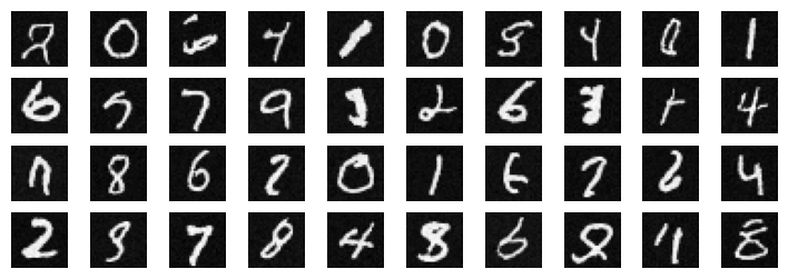
Epoch 20
The last thing left to do is add class-conditioning so we can prompt the U-Net to generate a certain class of images. We use similar fully-connected blocks to embed the class one-hot label, and zero it out with some probability so that the model can learn to ignore it. Here is the training loss:
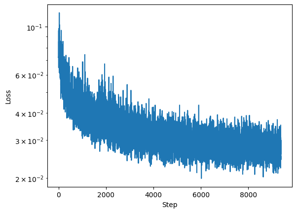
Class-Conditioned DDPM Training Loss
We use classifier-free guidance and sampling to visualize some results ($\gamma = 5$):
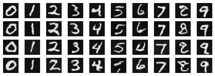
Epoch 5
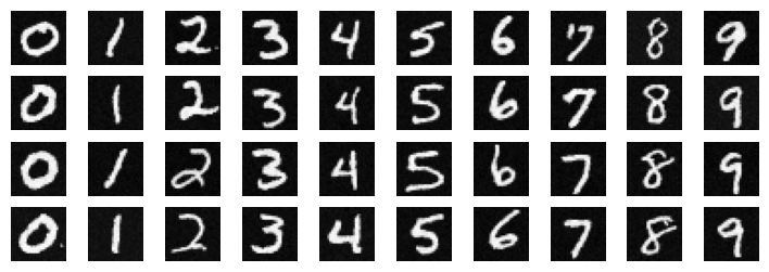
Epoch 20
This was absolutely the coolest project I've ever done at Berkeley and I'm so grateful to have had the opportunity to work on it. I learned so much about diffusion holy moly thank you for creating this!